ACTIVITY 12 Color Image Segmentation

In previous activities, the segmentation of the ROI from the background was done by binarization of the grayscale image. However, if the the grayscale image is similar to that shown below, it would be hard choose a threshold value which can properly separate the ROI from the background. Thus, new techniques of segmentation are introduced in this activity: parametric and nonparametric. There is no need to convert the truecolor image into a grayscale image. The histogram of the RGB values will be used to separate the ROI from the background.


Before proceeding with the segmentation process, the variation in the brightness level of the 3D objects were dealt with first. Brightness information can be disregarded if the RGB values are normalized to the intensity values at each point. That is, the RGB values at a point are divided by the sum of the of the RGB values at that point. This color space, which contains only chromaticity/color information, is called the normalized chromaticity coordinates or NCC. Figure 1 shows the NCC where the x-axis is r and the y-axis is g. b need not be shown here because its value can already be derived from r and g.

Parametric segmentation is done by assuming that the probability distribution function (PDF) of the image is a Gaussian distribution independent along r and g. The Gaussian PDF equations, form shown in the manual, for r and g are established by getting the mean, standard deviation and variance of the rg values of the ROI, which must be a monochromatic patch. The probability values along r and g are then multiplied and the product is already the correlation between the color information of the points in the image and the ROI. The process of segmentation is done by determining the probability that the rg values at points in the image belong to the color distribution of the ROI. This means the portion in the image that has the same color as the ROI, or high probability, will appear as bright spots in the resulting segmented image.

In nonparametric segmentation, no form of PDF is assumed and the 2D histogram of the binned rg values is used. The histogram is a N x N matrix where N is the number of bins. A sample code of creating a 2D histogram is shown in the manual. The process of segmentation is done by histogram backprojection. That is the pixel locations are assigned with new values depending on the r and g values. The new value is the value in the 2D histogram of the (r*N, g*N) location. Bright spots correspond to the portions of the image with the same color information as the ROI.

Figure 1. Resulting images after nonparametric and parametric segmentation of the patches of the sample images (third and last column). The patches are the small images just above the sample images. The second column consists of the 2D histogram of the patches.

Figure 1 shows several examples of nonparametric and parametric segmentation (third and last columns, respectively). The first four images illustrate how the segmentation process can also be used to highlight only the portions in a monochromatic object that have the same shade as the patch. The variation in the color of a 3D object is also evident in these results. The fifth image is a clear proof that the techniques used can properly segment the ROI from the background without having to convert the image into grayscale. The succeeding images segment the fruits in the image having the same color as the patch. The colors may not be exactly the same. As long as the fruit has r or/and g values, which are more or less the same as that in the patch, that fruit will be highlighted in the segmented image. The correlation in the in the r and g values of the image and the patch is illustrated in the variation of brightness of the highlighted spots. The nearer the color of the fruit to the color of the patch, the brighter the highlighted spots will be.

The created 2D histograms were checked by comparing the bright portions in the histogram with the NCC plot above. It can be seen that the bright portions are located at the same position as the location in the NCC plot of the color of the patch.

Comparing the results of parametric and nonparametric segmentation, it can be seen that the former is a better technique of highlighting portions that have color more or less the same as the patch. The trace of the fruits in the segmented image is more solid when the former technique is used as compared to when the latter technique is used. This is probably because the Gaussian distribution generates higher probability than when using the 2D histogram of the patch. However, it must be noted that the number of bins used for the parametric segmentation above is 256. This means the colors/shades of colors are highly separated, and so fewer portions in the image will be detected having the same color as the patch. This explains why in the results above the parametric method has darker and fewer highlighted spots than the parametric method. Figure 2 shows the different results when different number of bins is used. It can be seen that more fruits are highlighted when the bin is just 10. The trace is even more solid than the trace using parametric method. This is because with smaller bins, more colors of the same shade are grouped. From the results below, it can be seen that using 100 bins gives us the best result for highlighting only the fruits that have exactly the same color as the patch.

Figure 2. Parametric segmentation of the banana and grape patches using different bins (10, 100, 256).

I would like to thank Thirdy, Master and all other who have helped me understand what has to be done for this activity. I would give myself a grade of 10 for a job well done (according to me).

References:

1. Orange image: http://msp256.photobucket.com/albums/hh194/yehitsroger/orange.jpg
2. Mango: http://carinderia.net/blog/wp-content/uploads/2008/12/mango13.jpg
3. Green Apple: http://2.bp.blogspot.com/_wxeBei5m--0/SeaZnk8DBfI/AAAAAAAAARE/uci2eKrBTtU/s400/apple_green_fruit_240421_l.jpg
4. Red Apple: http://www.ableweb.org/news/winter2009/images/fruitApple1c4.jpg
5. Fruits: http://files.myopera.com/buksiy/albums/739313/Fruits.jpg
6. Apple Tree: http://www.kevinecotter.com/appletree.jpg

ACTIVITY 11 Color Camera Processing

The main goal for this activity is to balance unbalanced images using white patch (WP) and gray world (GW) algorithms. The image is unbalanced if the portions that are supposed to be white do not appear white. Just like the images in Figure 1, the supposedly white portions appear bluish. This means the images are captured using a WB setting not appropriate for the lighting conditions of the room/surroundings.

White patch algorithm divides all RGB values with the RGB values of the supposedly white portions. In doing so, these portions are forced to have a value of 1 producing a true white color. In this case, the bluish color can be thought of as an offset of the white color. Forcing the bluish color to be white allows the rest of the colors to be rendered correctly with respect to the white color. The balanced images using WP algorithm appear darker in Figure 1 (second column) because a constant (< style="text-decoration: underline;">

Figure 1. White balancing of unbalanced images. First column: unbalanced images; second column: using white patch algorithm; third column: using gray world algorithm.

Figure 2. White balancing of unbalanced images. First column: unbalanced images; second column: using white patch algorithm; third column: using gray world algorithm.

Figure 3 below shows the balancing of an image containing only a single hue. The resulting images show that WP algorithm produces better results than GW algorithm. Unlike in the multicolor images (Figures 1 and 2), the single hue introduces a bias in the balancing of the image. The yellowish color in the balanced image of GW algorithm is due to the bias in the red color since the mean of the whole image (mostly red) is used and not just of the white portion.

Figure 3. The white portion inside the black circle is the white patch used.

Figure 4. White balancing of an unbalanced image with single hue. First column: unbalanced images; second column: using gray world algorithm; third column: using white patch algorithm.

For this activity, I would give myself a grade of 10 because I was able to balance the images using both algorithms and explain the results I got. Thank you to Thirdy and all those who lent me their things for the photoshoot.

ACTIVITY 10 Preprocessing Text

The available image is titled, so it has to be rotated first using the mogrify() function in SciLab. Figure 1 shows an example of a cropped image and the resulting image after rotating it by 1.21 degrees. A disadvantage of rotating the image is the resulting image has lower resolution or blurry.

Figure 1. Rotation of the image.

Figure 2 shows the resulting images after applying a technique on the original image or the processed image. The first image is the inverted image of the original image (black becomes white and vice versa). Inversion of the image makes the choosing of the threshold value in the binarization of the image much easier. To remove the horizontal line between the texts ‘DEMO III’ and ‘Position’, a filter mask (vertical line with a hole at the center) was multiplied to the Fourier transform of the image. This technique is simply linear filtering in the Fourier/frequency domain. The resulting image is already clean, i.e., texts well separated from the background, so no further processing needs to be done. To make the texts one-pixel thick, the thin() function is applied to the image. Looking at the results, it can be observed that the characters in the word 'Position' are not highly resolved probably because the the spacing is too small that they seem to be connected. The failure to extract the letters in their complete form is due to the uneven brightness of the lines forming the letters. Making the texts one-pixel thick worsens their reconstruction. This is because of our failure to extract the letters completely, as well as clearly separate from each other.

Figure 2. Processing of the 'DEMO III, POSITION' text in the image.

The next figure demonstrates the processing of plain handwritten texts in a cropped image of the form. Again, the image is inverted first and then the horizontal lines are removed by linear filtering in the Fourier domain using the same filter mask. Since the binarized image is not yet that clean, it is further processed by applying the morphological operation opening on the binarized image. The texts are then made one-pixel thick. The reconstruction is still not good especially in the one-pixel thick texts. It is not possible to discern what these letters are using the results of our reconstruction. This is mainly because of the indecipherable handwriting of the person writing these texts. Acually, the reconstruction is good if we just look at the original image and not considering that these are supposed to be letters. If we think of the texts as just lines or curves, then we can say that the reconstruction is good. To illustrate how the labeling of the letters could have been done fo perfectly reconstructed texts, Figure 4 is shown below.

Figure 3. Processing of the handwritten texts in the image.

Figure 4. Labeling of the texts.

For this part of the activity, we counted the number of times the word 'DESCRIPTION' appeared in the image. We did it by using the correlation function we have learned in activity 5. The technique to have a good correlation when the word appears is to binarize the image and the template using the same threshold value. The word in the template must also be located at the center to be able to project the correct location of the words in the image of correlation values. Since there are three 'DESCRIPTIONs' in the image, there appear three very bright small dots in the image of the correlation values. Figures 5 and 6 show the location of the words in the image and the location of the bright spots in the image of correlated values, respectively.

Figure 5. Encircled 'DESCRIPTION' in the image.

Figure 6. Instances of the word 'DESCRIPTION' in the image.

I would like to thank Thirdy, Mandy, Jaze, Gilbert, Rommel, Alva and all others who have helped me understand this activity. I would give myself a grade of 10 because I was able to generate the necessary results and explain them.

ACTIVITY 9 Binary Operations

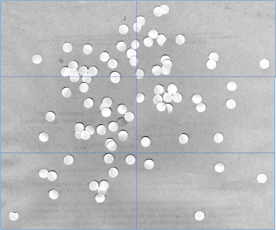
The purpose for this activity is to learn the techniques of properly segmenting/separating the region of interest (ROI) from the background. One technique is the binarization of the image. However, this method is not enough sometimes especially when there is an overlap in the graylevel distribution of the background and the ROI. One way to improve the separation of the ROI from the background using this technique is by creating subimages. The goal would be to have less ROI in the subimage to avoid the overlapping in the graylevel distribution. The threshold value may differ for the different subimages. This means the more the subimages are, the higher the success that the ROI will be well segmented from the background.

Unfortanately, binarization even with so many subimages is still not enough. A technique can be employed in the binarized subimages to further clean them. This is with the use of the morphological operations we learned in the previous activity, i.e., erosion and dilation. For this activity, we will be using new operations which utilizes both erosion and dilation. Opening is the operation in which the image is eroded first, and then the result is dilated using the same structuring element (SE) or another one. Closing, on the other hand, is the operation that dilates first, and then erodes the resulting image.

Proper segmentation is required especially when dealing with image-based measurements. For example, in this activity, we would like to calculate the area of the circles/holes. To be able to arrive at an accurate value, the image has to be prepocessed first.

The following were done to have a well-segmented ROI from the background:

1.) The images were subdivided into 6 subimages. (see Figure 1)

2.) For each subimage, the histogram was generated. (see Figure 2)

3.) Choosing a threshold value for each subimage (~0.80), the subimages were binarized. (see Figure 3)

4.) The binarized images were then further cleaned using only the opening function. (see Figure 4) I didn't find the closing function usefeul becauses it does not separate nearly connected blobs but instead treat them as one blob. On the other hand, using both opening and closing functions do not give that much difference in the calculation of the area.

5.) The blobs in the each subimage are then labeled using the function bwlabel(). It simply assigns an integer number to all connected pixel locations. Different groups of connected pixels have different assigned values. (see Figure 5)

6.) The area of each blob in the subimage is then calculated. This was done by simply getting the size of the blob with that assigned integer number. A bar graph of the calculated areas arranged in decreasing order is then established (see Figure 6) Extreme values are not included in the calculation of the mean area and standard deviation. In this case, only data 10-52 are included. The calculated mean area is 521 pixels while the standard deviation is 23.

Figure 1. The image subdivided into 6 parts.

Figure 2. Histogram of the subimages.

Figure 3. Binarized form of the subimages.

Figure 4. Resulting image after applying the opening function on the subimages.

Figure 5. Labeled holes of the subimages.

Figure 6. Calculated areas arranged in decreasing order.

I would give myself a grade of 10 for this acitvity because I believe I did this activity correctly. I would like to thank Thirdy and Jaze for their help in some parts of this acitivity.